MATH 315 Fall 2024
MATLAB Exploratory 1
Computer Modeling
of Plant Growth
If you have not already done so, download and
install MATLAB on your own computer. Click here
for details on how to do this. Review the basic features of MATLAB. The Getting Started with MATLAB video
should be useful.
The name MATLAB stands for Matrix Laboratory.
The American mathematician Cleve Moler
(born August 17, 1939) created MATLAB in the late 1970’s to assist his
students at Stanford and the University of New Mexico. Moler
cofounded the company MathWorks to commercialize this software. The MathWorks website features
hundreds of useful links.
In this exploratory,
we will focus on the foxglove (Digitalis
purpurea) example 10.3 of Causton. Recall that
the number, y, of plants surviving at
time t (measured in months from the
emergence of the seedlings) was given by the equation
![]()
Show first (paper and pencil
exercise) that
![]()
and
hence that y satisfies the differential equation
![]() with yo = y(0) =100.
with yo = y(0) =100.
Rewriting the differential equation
as
![]()
we observe that the foxglove
population decreases at a constant
percentage rate.
Conversely, you saw in first year
calculus, that if y is any quantity
that grows (positively or negatively) at a constant percentage rate, so
that y
satisfies the equation y'/y = k,
then y must have the form ![]() (You may wish to review, at your
leisure, the derivation of this fact).
(You may wish to review, at your
leisure, the derivation of this fact).
We
are going (temporarily!) to forget this little bit of mathematics and use MATLAB to investigate the behavior of
the foxglove population, assuming only that its initial population is 100 and
that it decreases at a constant percentage rate, 23.1%. MATLAB
has the capacity to solve analytically many commonly occurring
differential equations producing a closed form answer. Most differential
equations arising as models of real world situations,
particularly nonlinear systems, do not possess closed form answers we can
find. Thus, algorithms to provide
approximate numerical solutions are critically important. MATLAB
has many different numerical
methods built in, some of which we will explore in this course. For now, we
will focus on perhaps the simplest scheme: Euler’s Method.
The Euler method This
method, introduced by the great Swiss mathematician Leonhard Euler (1707
-1783), is based on a simple geometric interpretation of the derivative.
Suppose
that u = f(t) is a differentiable function of t and that the value of the function and its first derivative are
known at a number t0 . We wish to approximate the value
of the function at a nearby number to +
∆t. Direct computation may be quite
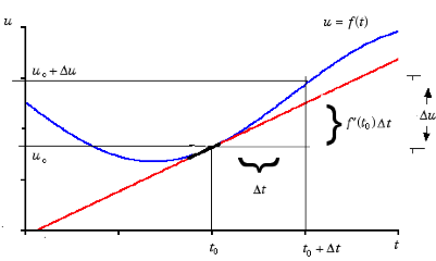
difficult. Note, however, that the graph of the tangent line to the curve u = f(t)
stays close to the curve near a point of tangency (to,f(to))
= (to, uo). The slope of the tangent line is given as f'(to) = u'(to, uo).
It is a simple matter to use the equation of the tangent line to find the
point on that line with first coordinate equal to to + ∆t. If ∆t is small, then the second coordinate of this point is a good
approximation to the value f(to + ∆t ) since the tangent line will not
wander far from the curve (see Figure 1 below). The smaller ∆t is, of course, the better the
approximation will be. Analytically, the actual change in the function from to to to +
∆t is
∆u = f(to
+ ![]() ) - f(to) = f(to +
) - f(to) = f(to + ![]() ) -f(to)
) -f(to)
The approximation is that ∆u is roughly equal to f '(to ) ![]() so that
so that
f(to + ![]() ) ~ uo + f
'(to)
) ~ uo + f
'(to) ![]()
which may also be written as
f(to + ∆t) ~ uo + u'(to ,
uo ) ∆t,
where ~ is a symbol representing
"approximately equal to."
 s\
s\
Figure 1.
We approximate the change in height of the graph of a function near the point
of tangency by the change in height of the tangent line. '
___________________________________________________
EXAMPLE
Suppose u = f(t) = and to = 4. Then
uo = = 2 and f'(t) = so that f'(to) = f'(4) =
u'(4,2) = = . The
approximation that is made here is
~ 2 + ∆t
If we wish to compute for
example, then we take ∆t = .41. The
approximate value is 2 + = 2.1025. The actual value of is 2.100.
The approximation here is quite good.
___________________________________________________
Many
calculus texts contain detailed discussion of this method of
"increments" for approximations. See, for example, Section 2.8,
“Linear Approximations and Differentials” in Swokowski,
Olinick and Pence’s Calculus, Sixth Edition (Boston: PWS, 1994).
The
method of increments is the basis for Euler's technique of approximating
solutions to differential equations.
In the context of the foxglove model, ![]() which has the form
which has the form ![]() suppose the initial level of foxgloves is y0. Then the rate of change is
suppose the initial level of foxgloves is y0. Then the rate of change is ![]() . In a short time
interval ∆t, the amount ∆y that the foxglove population will
change is approximately
. In a short time
interval ∆t, the amount ∆y that the foxglove population will
change is approximately ![]()
Thus at
time t1 = to + ∆t = 0 + ∆t = ∆t, the new foxglove population level will be approximately
![]()
If we
choose ∆t to be small, then the estimated
coordinates will be quite close to the actual coordinates at time ∆t.
Once a new population has been
estimated, it may be treated as the initial point of the system and the method
of increments can be applied again. This may be done as often as you like. The
general formula for estimating successive populations would be
![]()
![]() t
t
1.
Your
first task is to create a MATLAB program to implement Causton’s example. Choose a step size ![]() of 1 to begin and plot the numerical
approximation over the time interval from 0 to 15 months. Compare the plot of
the numerical approximations to the plot of the actual solution.
of 1 to begin and plot the numerical
approximation over the time interval from 0 to 15 months. Compare the plot of
the numerical approximations to the plot of the actual solution.
It should be fun to create a LiveScript from scratch,
but if you get stuck, you might modify the MATLAB file Euler_Method_Example.mix which you can download from the Handouts
folder on our course website.
2.
Run your program with some smaller and
larger sizes for ![]() (suggestions: .025, .001, 2.0) and
compare the results.
(suggestions: .025, .001, 2.0) and
compare the results.
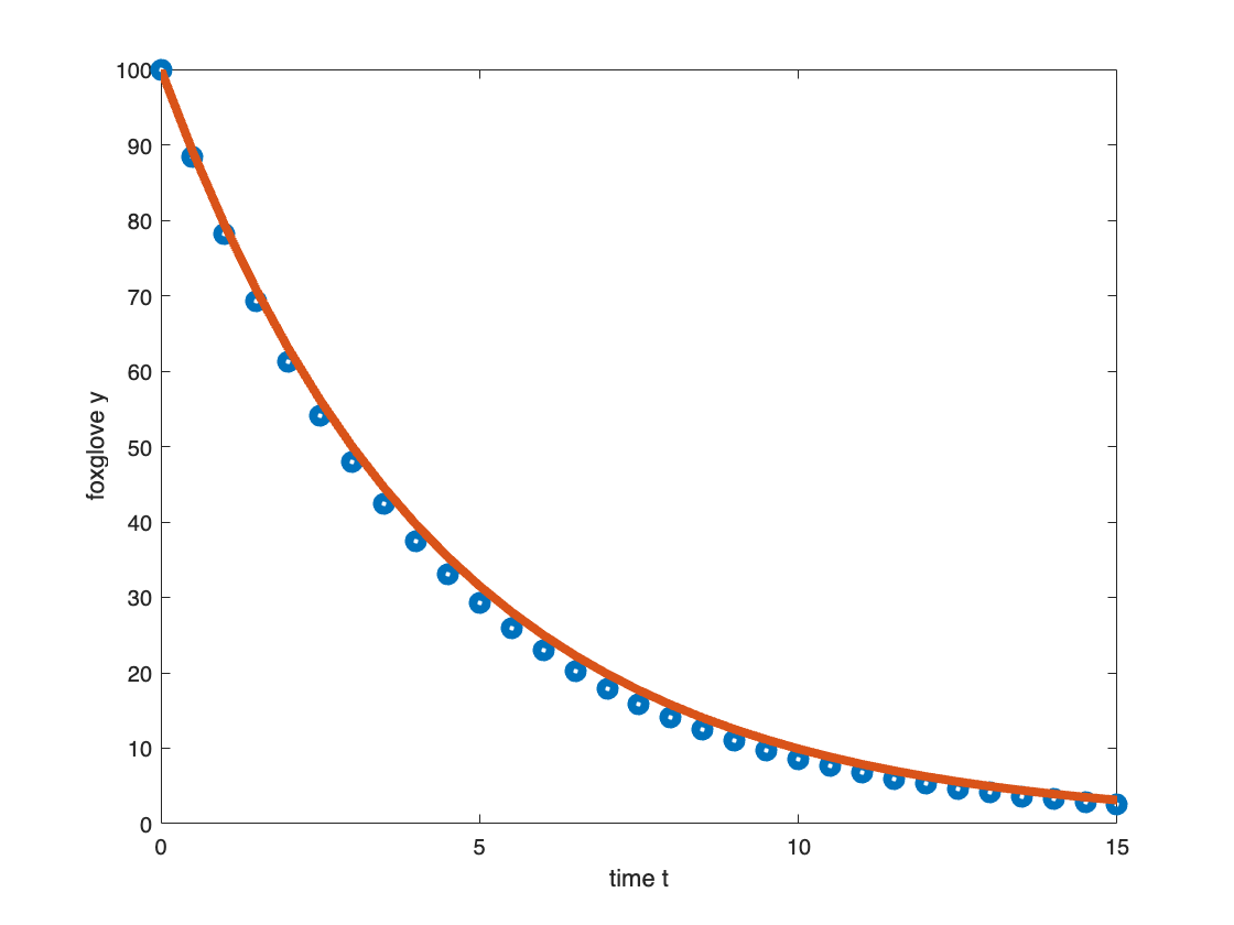
3.
For ![]() = 0.5, display a plot which shows the graphs
of the Euler Method estimated values and the exact values for the foxglove
population. Your plot will probably look something like
= 0.5, display a plot which shows the graphs
of the Euler Method estimated values and the exact values for the foxglove
population. Your plot will probably look something like
For ![]() = 0.5, display a table which shows the Euler
Method estimated values and the exact values for the foxglove population at
each month. Your table will probably look something like
= 0.5, display a table which shows the Euler
Method estimated values and the exact values for the foxglove population at
each month. Your table will probably look something like
|
|
Month |
Estimated_Foxglove |
Exact_Foxglove |
|
|
0 |
100 |
100 |
|
|
1 |
78.234 |
79.374 |
|
|
2 |
61.206 |
63.002 |
|
|
3 |
47.884 |
50.007 |
|
|
4 |
37.461 |
39.693 |
|
|
5 |
29.307 |
31.506 |
|
|
6 |
22.928 |
25.007 |
|
|
7 |
17.938 |
19.849 |
|
|
8 |
14.033 |
15.755 |
|
|
9 |
10.979 |
12.506 |
|
|
10 |
8.5893 |
9.9261 |
|
|
11 |
6.7197 |
7.8788 |
|
|
12 |
5.2571 |
6.2537 |
|
|
13 |
4.1129 |
4.9638 |
|
|
14 |
3.2177 |
3.94 |
|
|
15 |
2.5173 |
3.1273 |
4. Renewing the population. New
foxgloves may be added to the population by external forces (a gardener, for example) Investigate
the number of living foxglove plants if the gardener adds 10 new plants each
month. The differential equation
representing this situation would be ![]() Without solving the differential equation,
show that
Without solving the differential equation,
show that ![]() Modify your MATLAB file to use Euler’s Method
to plot the estimated foxglove over a long period of time. Do some simulations
with initial y value well above 43.29 and others with a much smaller
positive value below 43.29.
Modify your MATLAB file to use Euler’s Method
to plot the estimated foxglove over a long period of time. Do some simulations
with initial y value well above 43.29 and others with a much smaller
positive value below 43.29.
5. Explain why ![]() and
and ![]() are not solutions of the differential
equation
are not solutions of the differential
equation ![]() . Use techniques from elementary
calculus to find a correct closed form solution. You can also find a solution
method in Chapter 2 of the Brannan & Boyce differential equations text.
. Use techniques from elementary
calculus to find a correct closed form solution. You can also find a solution
method in Chapter 2 of the Brannan & Boyce differential equations text.
If you are anxious to learn more about
other numerical methods for solving differential equations, take
a look at Chapter 8 of Brannan and Boyce.